Reshaping Data: Join, Stack, Aggregate, Dedup & Sample

Until now we've worked with a single, tidy table. Reality is messier. Your sales sit in one file, one row per order. The details about each store — its region, type, and size — sit in another. To answer a question as basic as "which region earns the most revenue?", you first have to bring those tables together, then summarize them to the right level of detail. This is data reshaping, and it's where a lot of analysis quietly happens.

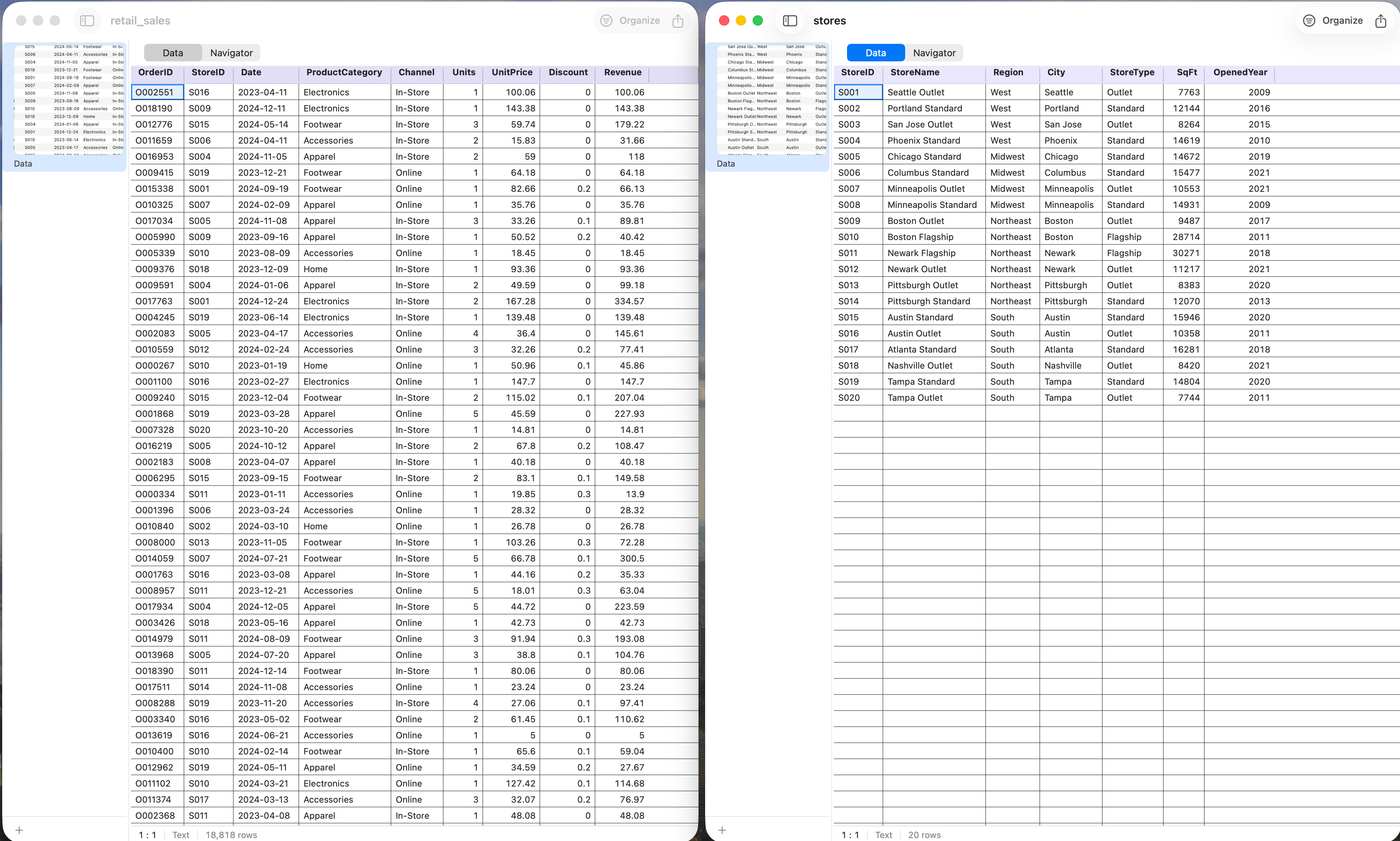
We'll switch datasets for this lesson, because reshaping only makes sense with relational structure: a fact table of retail orders and a dimension table of stores, linked by a shared StoreID.

Joining two tables

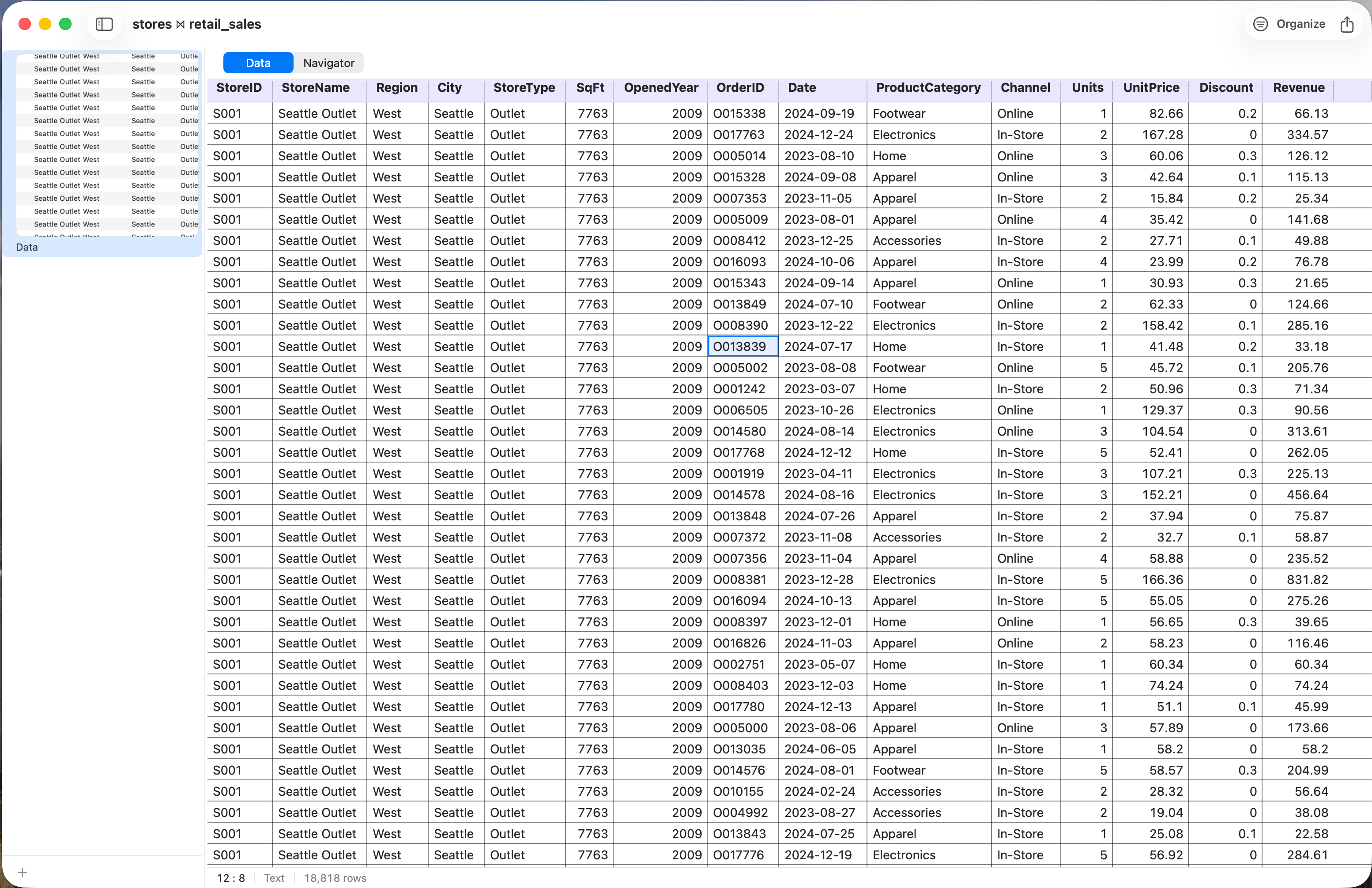
A join matches rows from two tables on a shared key. Here, joining the sales table to the stores table on StoreID stitches each store's attributes onto every order line — so each sale now knows its region, store type, and city.

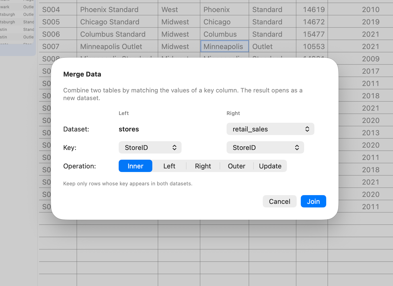
The join type matters. An inner join keeps only rows that match in both tables. A left join keeps every row from your primary (left) table, filling in blanks where the other table has no match. For analysis you usually want a left join from the fact table — that way you never silently drop a sale just because its store record happens to be missing.

Adding group-level statistics

Now you can answer the revenue question. Aggregate Data computes a statistic for each group and writes it back as a new column. Pick one or more value columns (the parameters), choose the columns to group by — here Region and ProductCategory — and pick a statistic, say the sum. Stratum adds a column holding each group's total Revenue; you can repeat that value on every row in the group, or place it on just the first row of each group.

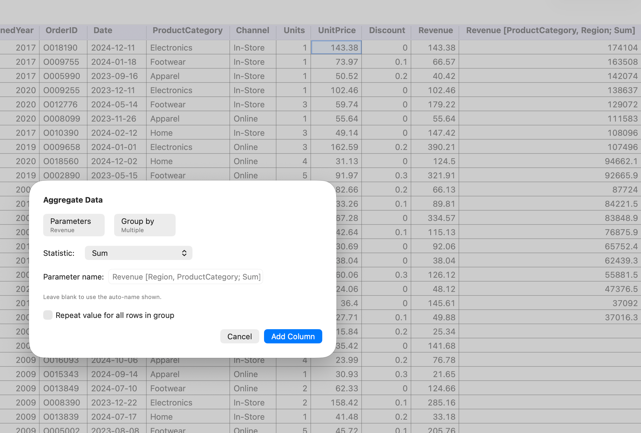
It's one statistic per run: to also see the average Discount or a row count per group, run Aggregate again with that statistic selected. Choosing the group keys and the statistic is the analysis — summing Revenue measures the business outcome, averaging Discount describes pricing behavior, and a count tells you how much each figure rests on.

Want several statistics side by side in one place? That's what the Summary report is for — it breaks one or more measures down by your grouping columns (sums, means, counts and more) as a single pivot you can read or export.

Cleaning up: dedup and sample

Two more operations round out the toolkit. Deduplication guards against double-counting: define the columns that make a row unique — here, OrderID — and keep the first or last occurrence. Run on a clean order table, it doubles as an integrity check (you'd expect zero duplicates).

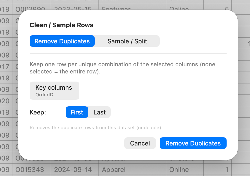
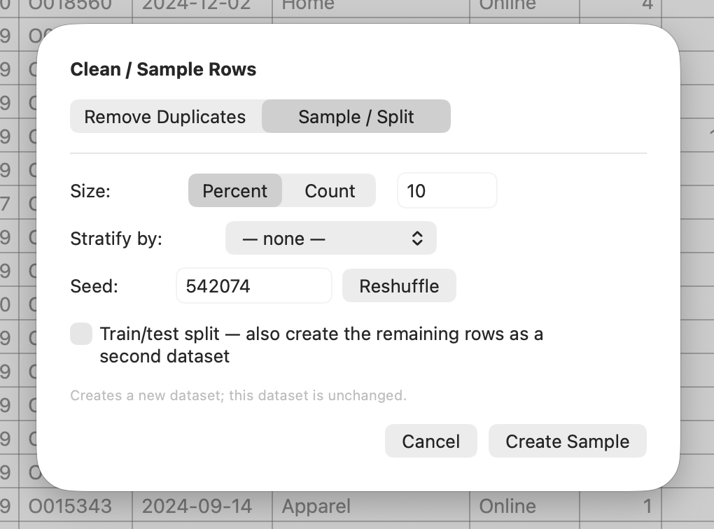
Sampling draws a random subset. A 10% sample makes iteration fast while you're exploring, and because the rows are chosen at random — not just the first N — the subset stays representative of the whole.

With data imported, derived, filtered, and reshaped, the groundwork is done. From the next lesson on, we turn to seeing and testing — starting with the chart that begins almost every analysis: the histogram.