Multiple Regression That Isn't Fooled by Confounders

A single-variable comparison is easy to fool. Multiple regression is how you hold everything constant at once and ask a fair question. Here's a real, worked example where adding one variable to the model doesn't just improve the fit — it reverses the conclusion.

Follow along: diamonds — 53,940 real diamonds (carat, cut, color, clarity, dimensions, price), the public ggplot2 dataset. Download the CSV and rebuild every model below in Stratum — no code required.

The wrong answer a simple model gives

Start naïve. Regress diamond price on cut quality alone. The result:

R² = 0.018.

Not 8% — under one percent. Cut, in isolation, explains almost nothing about price. Worse, if you read the coefficients, they suggest better cuts are associated with lower prices. Ship that and you'd report that cut quality is irrelevant, maybe even harmful to value. Both conclusions are wrong, and the reason is a lurking variable — size — that the one-variable model has no way to account for. (The full story on why is a classic case of Simpson's paradox.)

Adding the confounder changes everything

Now put size in the model. Because price scales with carat as a power law, we use log(price) and log(carat) (why log-transform). Watch the R² as we build up:

Model	R²
cut only	0.018
log(carat) only	0.933
+ cut	0.936
+ cut + color + clarity	0.983

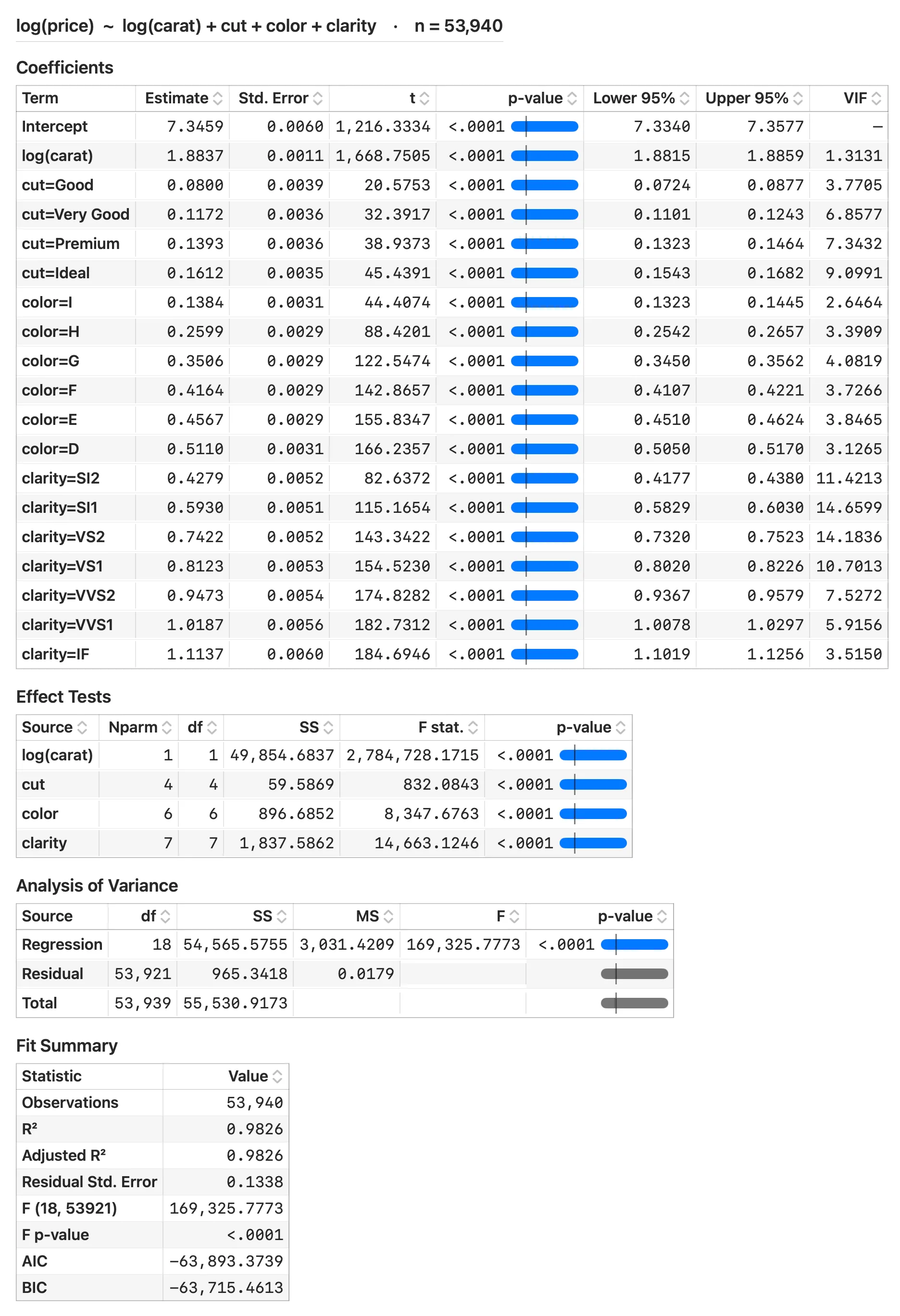
Coefficient table and R-squared climbing as size, cut, color, and clarity are added to the diamond price regression in Stratum — The R² climbs from under 2% to 98.3% as each of the four Cs enters the model — and the cut coefficients flip to their correct order.

Size alone explains 93% of the variation in price. That's the real driver the naïve model was blind to. And here's the crucial part: once size is in the model, cut starts competing fairly — comparing diamonds of the same size — and its coefficients flip to the correct order. Fair < Good < Very Good < Premium < Ideal, each grade now worth more than the last, exactly as a gemologist would predict. Same for color and clarity. The full four-C model explains 98.3% of price.

Why "controlling for" works

A multiple regression coefficient answers a specific question: holding every other variable in the model constant, what is the effect of this one? When you regress price on cut and carat together, the cut coefficient describes diamonds of equal carat — so the size confound can't leak into it. That's what "controlling for a variable" means mechanically. It's the regression equivalent of the binning trick (compare like with like), but it holds all the confounders still simultaneously, not one at a time.

This is why adding a variable can increase another variable's apparent effect, or reverse its sign. You're not just improving fit — you're changing the question from "what do Ideal diamonds cost?" to "what is Ideal cut worth for a stone of the same size, color, and clarity?" Those are different questions with different, and here opposite, answers.

Reading the model responsibly

A high R² is not a license to trust the coefficients. Two checks matter:

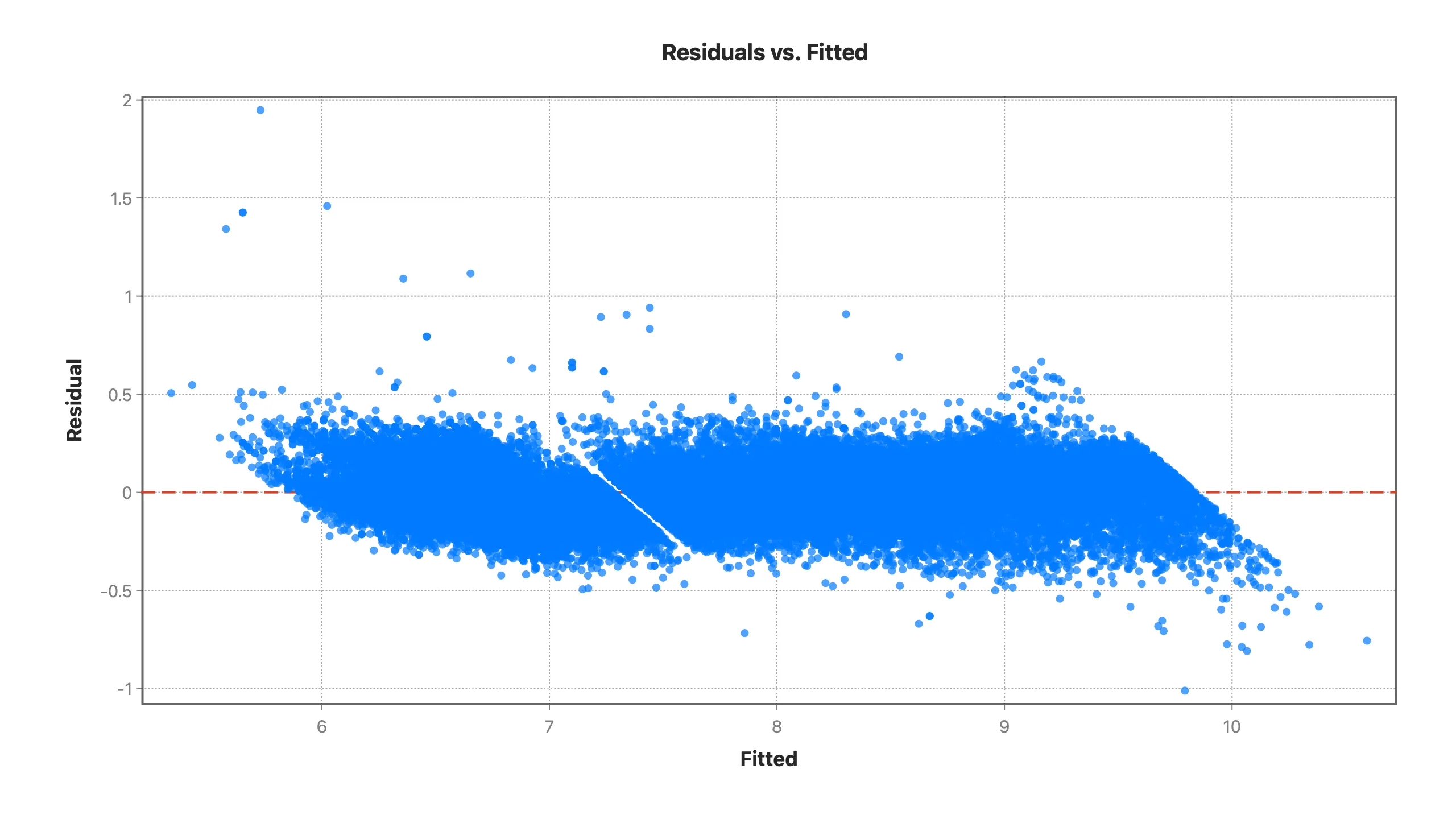
Residuals. Because we modeled log-price, the residuals sit flat and even — no funnel shape. If they fanned out, the standard errors (and every p-value) would be unreliable, and we'd say so.
What's not in the model. Regression only controls for confounders you actually include. The discipline is to ask, before trusting any coefficient, "what else differs that I haven't measured?" Here the four Cs plus size are a near-complete story (98.3%); in messier domains, unmeasured confounders are the permanent caveat.

Residuals-versus-fitted diagnostic for the log-price diamond regression, showing a flat, even band with no funnel shape — Residuals from the log-price model sit flat and even — no funnel — so the standard errors and p-values are trustworthy.

The takeaway

The difference between "diamond pricing is irrational" and "size explains 93% of price; cut is worth a precise premium at equal size" is one variable in a regression. Multiple regression isn't just a prediction tool — it's the instrument that lets you ask a fair question of observational data.

In Stratum you build this by adding variables to the model and watching the R², the coefficient table, and the residual diagnostics update together — no code, no matrix math.

Read the full Diamond Paradox analysis · Watch the walkthrough · Try Stratum free

Up next: Decision Trees on Real Data — when the relationships are non-linear and interactions matter, a tree finds the splits a regression would miss.